Julia で k-means クラスター分析

まず，驚くところは，Julia の k-means 関数では，データを ncol x nrow であたえるところ。
よく，help も読まないでやると，戸惑う所の騒ぎではない。
ということで，データを transpose して与えないといけない。
これくらいのこと，ユーザに強いるなよ！！

using RDatasets
iris = dataset("datasets", "iris");
a = Matrix(iris[!, 1:2]);
using Clustering, Plots
ncluster = 3;
R = kmeans(a', 3;  maxiter=200) # データを transpose して与えること！！！　a'  よりは，わかりやすく transpose(a) とする
a = assignments(R);
c = counts(R);
M = R.centers;
println(a) # 結果として，どこに分類されたか

[3, 3, 3, 3, 3, 3, 3, 3, 3, 3, 3, 3, 3, 3, 3, 3, 3, 3, 3, 3, 3, 3, 3, 3, 3, 3, 3 ...

M[1,:] # 各クラスターの平均値

3-element Array{Float64,1}:
 5.800000000000001
 6.823913043478258
 5.003921568627451

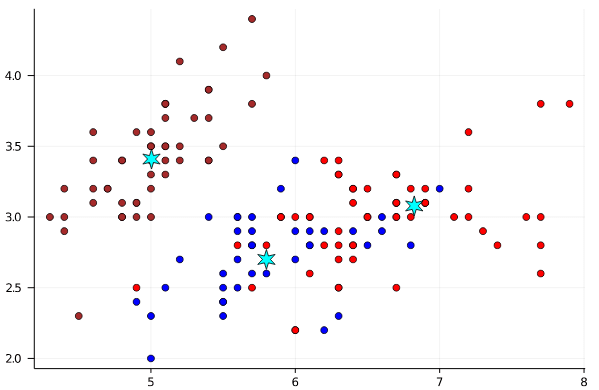
図に描いてみよう

repeateach(x, n) = vec([j for i = 1:n, j in x])
colors = repeateach([:brown, :blue, :red], 50);
p1 = scatter(iris[!, 1], iris[!,2], markercolor=colors, tick_direction=:out, label="");
p1 = scatter!(M[1,:], M[2,:], markershape=:star6, markersize=10, markercolor=:cyan, label="")
display(p1)

 

 

分類結果

using FreqTables

freqtable(iris[!, 5], a)

Out[7]:

3×3 Named Array{Int64,2}
 Dim1 ╲ Dim2 │  1   2   3
────────────────────────────
setosa        │  0   0  50
versicolor    │ 38  12   0
virginica     │ 15  34   1

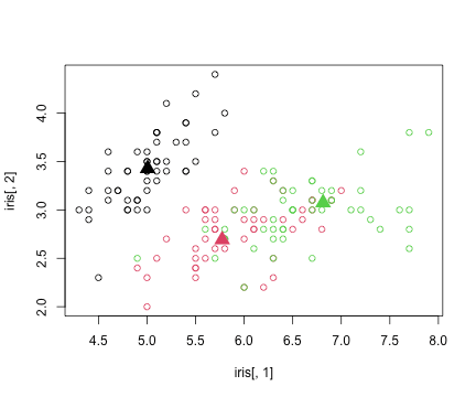
 R ではどんな風にやるのかな？？

using RCall

R"""
a = kmeans(iris[1:2], 3)
plot(iris[,1], iris[,2], col=rep(1:3, each=50))
points(a$centers, pch=17, col=c(1,3,2), cex=2)
"""

RObject{IntSxp}
            a$cluster
iris[, 5]     1  2  3
  setosa     50  0  0
  versicolor  0 38 12
  virginica   0 15 35

Julia のデータフレームで Query

直にデータフレームを操作するより楽なのかな？

using Query
using RDatasets
mtcars = dataset("datasets", "mtcars");
names(mtcars)

12-element Array{String,1}:
 "Model"
 "MPG"
 "Cyl"
 "Disp"
 "HP"
 "DRat"
 "WT"
 "QSec"
 "VS"
 "AM"
 "Gear"
 "Carb"

@collect で，条件に合ったものをデータフレームとして返す。

q1 = @from i  in mtcars begin
    @where i.AM == 1
    @select {i.Model, i.Cyl, i.MPG, i.WT}
    @collect DataFrame
end

13 rows × 4 columns

	Model	Cyl	MPG	WT
	String	Int64	Float64	Float64
1	Mazda RX4	6	21.0	2.62
2	Mazda RX4 Wag	6	21.0	2.875
3	Datsun 710	4	22.8	2.32
4	Fiat 128	4	32.4	2.2
5	Honda Civic	4	30.4	1.615
6	Toyota Corolla	4	33.9	1.835
7	Fiat X1-9	4	27.3	1.935
8	Porsche 914-2	4	26.0	2.14
9	Lotus Europa	4	30.4	1.513
10	Ford Pantera L	8	15.8	3.17
11	Ferrari Dino	6	19.7	2.77
12	Maserati Bora	8	15.0	3.57
13	Volvo 142E	4	21.4	2.78

 

普通のデータフレームになる。

using Statistics
cor(q1[!, 3], q1[!, 4])

-0.9089147883714981

cor(Matrix(q1[:, 2:4]))

3×3 Array{Float64,2}:
  1.0       -0.825998   0.847024
 -0.825998   1.0       -0.908915
  0.847024  -0.908915   1.0

@collect しなければ，イテレータを返す。

q2 = @from i  in mtcars begin
    @where i.AM == 1
    @select {i.Model, i.WT}
end

Model	WT
"Mazda RX4"	2.62
"Mazda RX4 Wag"	2.875
"Datsun 710"	2.32
"Fiat 128"	2.2
"Honda Civic"	1.615
"Toyota Corolla"	1.835
"Fiat X1-9"	1.935
"Porsche 914-2"	2.14
"Lotus Europa"	1.513
"Ford Pantera L"	3.17
⋮	⋮

... with more rows.

イテレータは for や 内包表記で使える。

for i in q2
    println("$(i.Model): weight is $(i.WT)")
end

Mazda RX4: weight is 2.62
Mazda RX4 Wag: weight is 2.875
Datsun 710: weight is 2.32
Fiat 128: weight is 2.2
Honda Civic: weight is 1.615
Toyota Corolla: weight is 1.835
Fiat X1-9: weight is 1.935
Porsche 914-2: weight is 2.14
Lotus Europa: weight is 1.513
Ford Pantera L: weight is 3.17
Ferrari Dino: weight is 2.77
Maserati Bora: weight is 3.57
Volvo 142E: weight is 2.78

[i.Model for i in q2 if i.WT > 2.5]

6-element Array{String,1}:
 "Mazda RX4"
 "Mazda RX4 Wag"
 "Ford Pantera L"
 "Ferrari Dino"
 "Maserati Bora"
 "Volvo 142E"

Julia と R のコラボレーションを jupyter notebook で記録

jupyter notebook というのは，いろいろな言語に対応している。

R の RStudio や，これまた多くの言語に対応している Atom と少し違って，スクリプトと実行結果をまとめて記録でき，成果物を LaTeX, PDF をはじめとして様々な形式で保存・閲覧できるという点で気に入っている。

たとえば，RStudio は，プログラム編集とコンソールとPlotなどのペインが分かれているので，作業しているときに煩わしい（別のやり方があるのかも知れないが）。その点，jupyter notebook はやったとおり，できたとおりのものが順に表示されていくので心地よい。あとで，不必要な部分や，追加処理を挿入するなどしてまとめて全部再度実行するのも簡単にできる。

 

それはさておき，今回は，Julia と R の環境を行き来して，いいとこ取りの分析環境を構築できるかどうか，ちょっとだけつまみ食いしてみよう。

以下では，jupiter notebook の結果を text ファイルに出力したまま（都合で html ファイルの一部分を切り取って）表示しているので不細工だが，本当は遙かに綺麗（そのまま出版できるレベル）なので，誤解なきよう。

 

まずは，Julia で，独立二標本の平均値の差の検定を行ってみる。
使うのは，ちょっと，長い名前だが UnequalVarianceTTest() だ。

 

In [1]:

using HypothesisTests

In [2]:

x = [2,1,3,2,4,3,2,3,4,5];

In [3]:

y = [3,2,3,4,5,6,3,2,3,3,3,4,3,2,6];

In [4]:

UnequalVarianceTTest(x, y)

Out[4]:

Two sample t-test (unequal variance)
------------------------------------
Population details:
    parameter of interest:   Mean difference
    value under h_0:         0
    point estimate:          -0.566667
    95% confidence interval: (-1.6209, 0.4876)

Test summary:
    outcome with 95% confidence: fail to reject h_0
    two-sided p-value:           0.2760

Details:
    number of observations:   [10,15]
    t-statistic:              -1.1192102478745312
    degrees of freedom:       20.56776717709893
    empirical standard error: 0.506309397848002

次に，Julia から RCall を介して，R の t.test() で同じデータを分析してみる

 

In [5]:

using RCall

長いスクリプトは，R""" と """ で挟んで，何行でも書ける。
$x, $y というのは Julia の x, y ということを表す。
結果を明示的に print() で書かないと，最後の出力しか表示されないので注意。

In [6]:

R"""
options(digits=15)
a = t.test($x, $y)
print(a)
print(a$statistic)
print(a$p.value)
"""

 

	Welch Two Sample t-test

data:  `#JL`$x and `#JL`$y
t = -1.119210247875, df = 20.5677671771, p-value = 0.275951369175
alternative hypothesis: true difference in means is not equal to 0
95 percent confidence interval:
 -1.620943659272958  0.487610325939624
sample estimates:
       mean of x        mean of y 
2.90000000000000 3.46666666666667 

                t 
-1.11921024787453 
[1] 0.275951369174595

Out[6]:

RObject{RealSxp}
[1] 0.275951369174595

In [7]:

R"a"

Out[7]:

RObject{VecSxp}

	Welch Two Sample t-test

data:  `#JL`$x and `#JL`$y
t = -1.119210247875, df = 20.5677671771, p-value = 0.275951369175
alternative hypothesis: true difference in means is not equal to 0
95 percent confidence interval:
 -1.620943659272958  0.487610325939624
sample estimates:
       mean of x        mean of y 
2.90000000000000 3.46666666666667 

図を描くと，図もその場に出力されるので快適。
ただ，希望しない出力もしてくれるのは大きなお世話ともいえるが，普通は気にしない分析結果なので，統計解析もしっかりやらなければならないよという戒めにもなるのかな？

In [8]:

R"""
group = rep(factor(c("x", "y")), c(length($x),length($y)))
value = c($x, $y)
a = boxplot(value ~ group)
"""

Out[8]:

RObject{VecSxp}
$stats
     [,1] [,2]
[1,]    1    2
[2,]    2    3
[3,]    3    3
[4,]    4    4
[5,]    5    5
attr(,"class")
        x 
"integer" 

$n
[1] 10 15

$conf
                 [,1]             [,2]
[1,] 2.00072025938679 2.59204575419949
[2,] 3.99927974061321 3.40795424580051

$out
[1] 6 6

$group
[1] 2 2

$names
[1] "x" "y"