#==========
Julia の修行をするときに,いろいろなプログラムを書き換えるのは有効な方法だ。
以下のプログラムを Julia に翻訳してみる。
主成分分析 http://aoki2.si.gunma-u.ac.jp/R/pca.html
ファイル名: pca.jl 関数名: pca
翻訳するときに書いたメモ
色々と凝って,機能が盛り沢山になった。
一般的に,計算精度の点からは SVD によるプログラムが推奨されるが,
たいていの場合は固有値・固有ベクトルによる結果と精度的に違いはない。
==========#
using CSV, DataFrames, StatsBase, Statistics, LinearAlgebra, Printf
# データフレームで与える
function pca(data::DataFrame; method="svd", center::Bool =true, scale::Bool =true)
pca(Array{Float64,2}(data); name=names(data), method, center, scale)
end
# 二次元配列で与える
function pca(data::Array{Int64,2}; name=[], method="svd", center::Bool =true, scale::Bool =true)
pca(Array{Float64,2}(data); name=[], method="svd", center=true, scale=true)
end
function pca(data::Array{Float64,2}; name=[], method="svd", center::Bool =true, scale::Bool =true)
nr, nc = size(data)
if length(name) == 0
name = "X" .* string.(1:nc)
end
if method == "svd"
# データ行列の特異値分解による主成分分析
temp = fit(ZScoreTransform, data, dims=1; center, scale)
data = StatsBase.transform(temp, data)
u, s, v = svd(data, full=false)
loading = v .* (transpose(s) ./ sqrt(nr-1))
score = u .* transpose(s)
eigenvalue = s .^2 ./ (nr - 1)
else
# 相関係数行列の固有値・固有ベクトルに基づく主成分分析
r = Symmetric(cor(data)) # 対称行列であることを明示するといいことがあるかも
eigenvalue, eigenvectors = eigen(r, sortby=x-> -x)
eigenvalue = [x < 0 ? 0 : x for x in eigenvalue]
loading = eigenvectors .* transpose(sqrt.(eigenvalue))
temp = fit(ZScoreTransform, data, dims=1)
data = StatsBase.transform(temp, data)
score = data * eigenvectors
end
signchange!(loading)
signchange!(score)
Dict(:method => method, :eigenvalue => eigenvalue,
:loading => loading, :score => score,
:name => name, :data => data, :center => center, :scale => scale)
end
# 主成分得点
predict_pca(object::Dict{Symbol,Any}) = object[:score]
predict_pca(object::Dict{Symbol,Any}, data::DataFrame) = predict_pca(object::Dict{Symbol,Any}, Array{Float64,2}(data))
function predict_pca(object::Dict{Symbol,Any}, data::Array{Float64,2})
temp = fit(ZScoreTransform, data, dims=1; center = object[:center], scale = object[:scale])
data = StatsBase.transform(temp, data)
rotation = object[:loading] ./ transpose(sqrt.(object[:eigenvalue]))
predict = data * rotation
signchange!(predict)
return predict
end
# 列ごとに見て,負の数が過半数のときは全体の符号を付け替え,常に正の数が過半数になるようにする
# 正負の数が同数の場合には,第1要素が負であれば全体の符号を付け替える
function signchange!(x::Array{Float64,2})
nr, nc = size(x)
half = fld(nr, 2)
for i = 1:nc
minus = sum(x[:, i] .< 0)
if minus > half || (minus == half && x[1, i] < 0)
x[:, i] = -x[:, i]
end
end
end
# サマリーの出力
function summary_pca(object::Dict{Symbol,Any}; npca::Int64=0)
function lineout(label, value)
@printf("%-16s", label)
for j = 1:npca
@printf("%10.5f", value[j])
end
println()
end
loading = object[:loading]
nc = size(loading, 1)
eigenvalue = object[:eigenvalue]
totalcontribution = sum(eigenvalue)
npca = npca == 0 ? sum(eigenvalue .> 1.0) : npca
eigenvalue = eigenvalue[1:npca]
loading = loading[:, 1:npca]
name = object[:name]
println("Principal Components Analysis")
@printf("%16s", "")
for j = 1:npca
@printf(" PC%02d", j)
end
println(" Contribution")
cum = sum(loading .^ 2, dims=2)
for i = 1:nc
@printf("%-16s", name[i])
for j = 1:npca
@printf("%10.5f", loading[i, j])
end
@printf("%10.5f\n", cum[i])
end
proportion = eigenvalue ./ totalcontribution .* 100
cumulative_proportion = cumsum(proportion, dims=1)
lineout("Eigenvalue", eigenvalue)
lineout("Proportion", proportion)
lineout("Cumulative Prop.", cumulative_proportion)
end
using Plots
# 主成分負荷量,主成分得点,倍プロット
function plot_pca(object::Dict{Symbol,Any}; axis1::Int64=1, axis2::Int64=2, col=:red, biplot=true, width=600, height=400)
function plotx(x1, x2)
plot(x1, x2,
seriestype = :scatter,
markercolor = col,
markerstrokecolor = col,
grid = false,
framestyle = :origin,
aspect_ratio = 1,
label = "",
xaxis = ("PC"*string(axis1), 0.5),
yaxis = ("PC"*string(axis2), 0.5),
title="Factor Scores")
end
function ploty(y1, y2, quiver2)
delta(y, len) = len / (maximum(y) - minimum(y)) / 1000
quiver2(zeros(nvariables), zeros(nvariables),
quiver = (y1, y2),
lc = :red,
grid = false,
framestyle = :origin,
aspect_ratio = 1,
label = "",
xaxis = ("PC"*string(axis1), 0.5),
yaxis = ("PC"*string(axis2), 0.5),
title = "Principal Component Loadings")
deltax = y1 .* (1 + delta(y1, width))
deltay = y2 .* (1 + delta(y2, height))
name = object[:name];
@. annotate!(deltax, deltay, text(name, :red, 8))
hline!([0], lc=:black, lw=0.5, label="") # ダミー:これがないと不都合発生
end
range(x) = (-abs(minimum(x)), abs(maximum(x)))
gr(size=(width, height))
loading = object[:loading]
score = object[:score]
x1 = score[:, axis1]
x2 = score[:, axis2]
y1 = loading[:, axis1]
y2 = loading[:, axis2]
minall = minimum(min.(y1, y2))
maxall = maximum(max.(y1, y2))
#delta = (maxall - minall) * 0.05
nvariables, npcas = size(loading)
rangex1 = range(x1)
rangex2 = range(x2)
rangey1 = range(y1)
rangey2 = range(y2)
ratio = max(maximum(rangey1./rangex1), maximum(rangey2./rangex2))
if biplot
px = plotx(x1, x2)
y1 = y1 ./ ratio
y2 = y2 ./ ratio
py = ploty(y1, y2, quiver!)
plot(py, label = "", title = "Biplot of PCA")
else
display(ploty(y1, y2, quiver))
display(plotx(x1, x2))
end
end
using Printf
# 名前付き配列出力
function dumplist(name::String, object::Array{Float64,2}; fmt="%10.5f")
nr, nc = size(object)
println("----- $name -----")
for i = 1:nr
for j = 1:nc
@eval(@printf($fmt, $(object[i, j])))
end
print("\n")
end
end
# 名前付きベクトル出力
function dumplist(name::String, object::Array{Float64,1}; fmt="%10.5f")
println("----- $name -----")
len = length(object)
for i = 1:len
@eval(@printf($fmt, $(object[i])))
end
print("\n")
end
data = [1 4 4 5
2 3 3 4
3 2 4 3
2 4 5 2
3 5 6 1];
object = pca(data);
obj2 = summary_pca(object);
#=====
Principal Components Analysis
PC01 PC02 Contribution
X1 0.63890 -0.75171 0.97326
X2 0.61824 0.76570 0.96852
X3 0.94686 0.23192 0.95033
X4 -0.95528 0.22267 0.96215
Eigenvalue 2.59953 1.25472
Proportion 64.98829 31.36810
Cumulative Prop. 64.98829 96.35639
=====#
object = pca(data, method="eigen");
obj2 = summary_pca(object);
#=====
Principal Components Analysis
PC01 PC02 Contribution
X1 0.63890 -0.75171 0.97326
X2 0.61824 0.76570 0.96852
X3 0.94686 0.23192 0.95033
X4 -0.95528 0.22267 0.96215
Eigenvalue 2.59953 1.25472
Proportion 64.98829 31.36810
Cumulative Prop. 64.98829 96.35639
=====#
# 行数より列数が多い場合
data = [3 1 2 3 4 3 5 5
5 3 3 5 4 3 4 3
2 4 1 2 2 3 4 2
1 5 3 2 3 4 2 1];
w = pca(data);
summary_pca(w);
#=====
Principal Components Analysis
PC01 PC02 Contribution
X1 0.84022 0.33659 0.81926
X2 -0.90864 0.17872 0.85757
X3 -0.02761 0.99104 0.98293
X4 0.72738 0.56788 0.85157
X5 0.71110 0.61763 0.88713
X6 -0.81255 0.45653 0.86865
X7 0.88495 -0.46553 0.99985
X8 0.90864 -0.17872 0.85757
Eigenvalue 4.83610 2.28843
Proportion 60.45130 28.60540
Cumulative Prop. 60.45130 89.05670
=====#
w0 = pca(data, method="eigen");
summary_pca(w0);
#=====
Principal Components Analysis
PC01 PC02 Contribution
X1 0.84022 0.33659 0.81926
X2 -0.90864 0.17872 0.85757
X3 -0.02761 0.99104 0.98293
X4 0.72738 0.56788 0.85157
X5 0.71110 0.61763 0.88713
X6 -0.81255 0.45653 0.86865
X7 0.88495 -0.46553 0.99985
X8 0.90864 -0.17872 0.85757
Eigenvalue 4.83610 2.28843
Proportion 60.45130 28.60540
Cumulative Prop. 60.45130 89.05670
=====#
long = Array{Float64,2}(transpose(data));
#=====
8×4 Matrix{Float64}:
3.0 5.0 2.0 1.0
1.0 3.0 4.0 5.0
2.0 3.0 1.0 3.0
3.0 5.0 2.0 2.0
4.0 4.0 2.0 3.0
3.0 3.0 3.0 4.0
5.0 4.0 4.0 2.0
5.0 3.0 2.0 1.0
=====#
l = pca(long);
summary_pca(l);
#=====
Principal Components Analysis
PC01 PC02 Contribution
X1 0.70648 0.59279 0.85052
X2 0.66205 -0.10838 0.45005
X3 -0.47141 0.79977 0.86186
X4 -0.96028 -0.03121 0.92311
Eigenvalue 2.08179 1.00376
Proportion 52.04472 25.09400
Cumulative Prop. 52.04472 77.13872
=====#
l0 = pca(long, method="eigen");
summary_pca(l0);
#=====
Principal Components Analysis
PC01 PC02 Contribution
X1 0.70648 0.59279 0.85052
X2 0.66205 -0.10838 0.45005
X3 -0.47141 0.79977 0.86186
X4 -0.96028 -0.03121 0.92311
Eigenvalue 2.08179 1.00376
Proportion 52.04472 25.09400
Cumulative Prop. 52.04472 77.13872
=====#
##################
using RDatasets
iris = dataset("datasets", "iris");
result = pca(iris[:, 1:4]);
result2 = summary_pca(result, npca=4);
#=====
Principal Components Analysis
PC01 PC02 PC03 PC04 Contribution
SepalLength 0.89017 0.36083 -0.27566 0.03761 1.00000
SepalWidth -0.46014 0.88272 0.09362 -0.01778 1.00000
PetalLength 0.99156 0.02342 0.05445 -0.11535 1.00000
PetalWidth 0.96498 0.06400 0.24298 0.07536 1.00000
Eigenvalue 2.91850 0.91403 0.14676 0.02071
Proportion 72.96245 22.85076 3.66892 0.51787
Cumulative Prop. 72.96245 95.81321 99.48213 100.00000
=====#
result = pca(iris[:, 1:4], method="eigen");
repeateach(x, n) = vec([j for i = 1:n, j in x])
colors = repeateach([:brown, :blue, :red], 50);
# バイプロット # savefig("biplot.png")
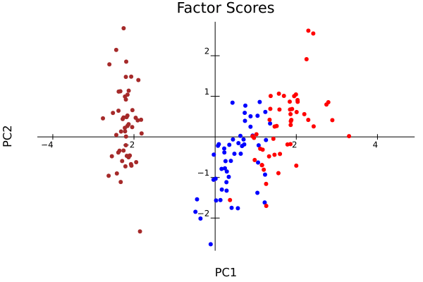
plot_pca(result, col=colors, width=600, height=600) # 主成分負荷量,主成分得点 # savefig("loadings_scores.png")
plot_pca(result, col=colors, biplot=false)
# 主成分負荷量,主成分得点 # savefig("loadings_scores.png")
plot_pca(result, col=colors, biplot=false)
 result_center = pca(iris[:, 1:4], center=true, scale=false);
summary_pca(result_center, npca=4);
plot_pca(result_center, col=colors, width=600, height=600)
result_scale = pca(iris[:, 1:4], center=false, scale=true);
summary_pca(result_scale, npca=4);
plot_pca(result_scale, col=colors, width=600, height=600)
result_center_scale = pca(iris[:, 1:4], center=false, scale=false);
summary_pca(result_center_scale, npca=4);
plot_pca(result_center_scale, col=colors, width=600, height=600)
half1 = vcat(iris[1:25, 1:4], iris[51:75, 1:4], iris[101:125, 1:4]);
half2 = vcat(iris[26:50, 1:4], iris[76:100, 1:4], iris[126:150, 1:4]);
repeateach(x, n) = vec([j for i = 1:n, j in x])
colors = repeateach([:brown, :blue, :red], 25);
res1 = pca(half1);
res2 = pca(half2);
summary_pca(res1, npca=2)
summary_pca(res2, npca=2)
plot_pca(res1, col=colors)
plot_pca(res2, col=colors)
result_center = pca(iris[:, 1:4], center=true, scale=false);
summary_pca(result_center, npca=4);
plot_pca(result_center, col=colors, width=600, height=600)
result_scale = pca(iris[:, 1:4], center=false, scale=true);
summary_pca(result_scale, npca=4);
plot_pca(result_scale, col=colors, width=600, height=600)
result_center_scale = pca(iris[:, 1:4], center=false, scale=false);
summary_pca(result_center_scale, npca=4);
plot_pca(result_center_scale, col=colors, width=600, height=600)
half1 = vcat(iris[1:25, 1:4], iris[51:75, 1:4], iris[101:125, 1:4]);
half2 = vcat(iris[26:50, 1:4], iris[76:100, 1:4], iris[126:150, 1:4]);
repeateach(x, n) = vec([j for i = 1:n, j in x])
colors = repeateach([:brown, :blue, :red], 25);
res1 = pca(half1);
res2 = pca(half2);
summary_pca(res1, npca=2)
summary_pca(res2, npca=2)
plot_pca(res1, col=colors)
plot_pca(res2, col=colors)


