Julia で主成分分析（その2）

色々な指定とか，順をおって自分でやらないといけないことが多くて使いにくいなあと。

include でもして，簡単に使える関数に仕立てた。以下の 12 行だけ。

julia> using CSV, DataFrames, Statistics, StatsBase, LinearAlgebra
julia> function pca(data::DataFrame; scale::Bool =true)
           pca(Array{Float64,2}(data); scale)
       end
julia> function pca(data::Array{Float64,2}; scale::Bool =true)
           r = Symmetric((scale ? cor : cov)(data))
           eigenvalue, eigenvectors = eigen(r, sortby=x-> -x)
           eigenvalue = [x < 0 ? 0 : x for x in eigenvalue]
           temp = fit(ZScoreTransform, data, dims=1; center=true, scale)
           score = StatsBase.transform(temp, data) * eigenvectors
           return eigenvalue, eigenvectors, score
       end

データの準備

julia> using RDatasets
julia> iris = dataset("datasets", "iris");
julia> data = iris[:, 1:4];

使うのは簡単。データフレームなり配列を関数に渡すだけ。この場合は，データを平均値 0，標準偏差 1 にしてから分析する。

データの中に単位の異なる変数が含まれている場合や，変数の分散の違いが分析に支障を生ずるような場合にはこちら（scale=true）でなければならない。

返されるのは固有値，固有ベクトル，主成分得点。全ての主成分を抽出して返すので，何個の主成分を使うかはご自由に。

julia> val1, vec1, score1 = pca(iris[:, 1:4]);

第 1 主成分と第 2 主成分で全体の 96% ほども説明できる。

julia> sum(val1[1:2])/sum(val1)
0.9581320720000164

図を描いてみよう。

julia> using Plots
julia> col = vcat(fill(:green, 50), fill(:blue, 50), fill(:red, 50));
julia> scatter(score1[:, 1], score1[:, 2], markercolor=col, label="")

分散・共分散行列を対象にする（データを標準偏差で標準化しない）場合は，scale=false を指定する。

julia> val2, vec2, score2 = pca(iris[:, 1:4], scale=false);
julia> scatter(score2[:, 1], score2[:, 2], markercolor=col, label="")

R のときは，このようになる。

julia> using RCall
julia> R"""
       ans1 = prcomp(iris[,1:4], scale.=TRUE)
       color = rep(c("chartreuse4", "blue", "red"), each=50)
       plot(-ans1$x[,1], -ans1$x[,2], pch=19, col=color)
       ans2 = prcomp(iris[,1:4], scale.=FALSE)
       plot(-ans2$x[,1], -ans2$x[,2], pch=19, col=color)
       """

Julia で主成分分析

最近は，主成分分析も機械学習の視点から使用されることが多いようだが，かなり違和感を感じる。

それはさておき，主成分分析の例示であるが，そのままでは Version 1.5.3 では動かないので，少し修正して掲載。

https://multivariatestatsjl.readthedocs.io/en/stable/pca.html

julia> using MultivariateStats, RDatasets, Plots
julia> plotly() # using plotly for 3D-interacive graphing
julia> iris = dataset("datasets", "iris"); # load iris dataset
julia> # split half to training set
       # 分析に使うデータ行列は列が観察値（つまり普通のデータ行列の転置！）
       Xtr = transpose(Array{Float64,2}(iris[1:2:end,1:4]));
julia> Xtr_labels = Array{String,1}(iris[1:2:end,5]);
julia> # split other half to testing set
       Xte = transpose(Array{Float64,2}(iris[2:2:end,1:4]));
julia> Xte_labels = Array{String,1}(iris[2:2:end,5]);
julia> # suppose Xtr and Xte are training and testing data matrix,
       # with each observation in a column
       # train a PCA model, allowing up to 3 dimensions
       M = fit(PCA, Xtr; maxoutdim=3)
PCA(indim = 4, outdim = 3, principalratio = 0.9957325846529409)
julia> # apply PCA model to testing set
       Yte = MultivariateStats.transform(M, Xte)
3×75 Array{Float64,2}:
  2.72714    2.75491     2.32396   2.65105     2.68917   …
 -0.230916  -0.406149    0.646374  0.0828144  -0.17411
  0.253119   0.0271266  -0.230469  0.0252853   0.231507
julia> # reconstruct testing observations (approximately)
       Xr = reconstruct(M, Yte)
4×75 Array{Float64,2}:
 4.86449  4.61087   5.40782   5.00775   4.90864   4.83689   …
 3.04262  3.08695   3.89061   3.39069   3.08963   3.35572
 1.46099  1.48132   1.68656   1.48668   1.48516   1.53664
 0.10362  0.229519  0.421233  0.221041  0.123445  0.300129
julia> # group results by testing set labels for color coding
       setosa = Yte[:,Xte_labels.=="setosa"]
3×25 Array{Float64,2}:
  2.72714    2.75491     2.32396   2.65105     2.68917   …
 -0.230916  -0.406149    0.646374  0.0828144  -0.17411
  0.253119   0.0271266  -0.230469  0.0252853   0.231507
julia> versicolor = Yte[:,Xte_labels.=="versicolor"]
3×25 Array{Float64,2}:
 -0.901049   -0.189593  -0.631938    0.737306   0.00578031  …
  0.350685   -0.7887    -0.40525    -1.01982   -0.74682
 -0.0027406   0.291058   0.0207768   0.121331  -0.179235
julia> virginica = Yte[:,Xte_labels.=="virginica"]
3×25 Array{Float64,2}:
 -1.4126    -1.95359   -3.35517   -2.89581   -2.8711    …
 -0.556727  -0.133821   0.692925   0.487134   0.828406
 -0.214115  -0.075898   0.293002   0.386084  -0.496979
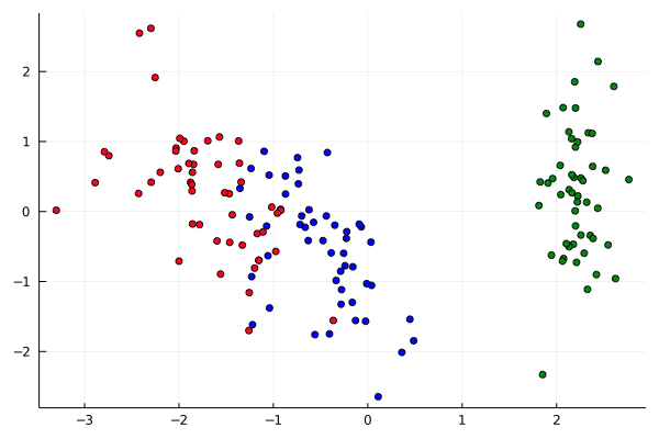
julia> # visualize first 3 principal components in 3D interacive plot
       p = scatter(setosa[1,:],setosa[2,:],setosa[3,:],marker=:circle,linewidth=0)
julia> scatter!(versicolor[1,:],versicolor[2,:],versicolor[3,:],marker=:circle,linewidth=0)
julia> scatter!(virginica[1,:],virginica[2,:],virginica[3,:],marker=:circle,linewidth=0)
julia> plot!(p,xlabel="PC1",ylabel="PC2",zlabel="PC3")

その他，fit(PCA,...) が返すオブジェクトの出力

julia> indim(M) # 入力データ行列の次元数（変数の個数）
4

julia> outdim(M) # 結果の次元数（抽出された主成分の数）
3

julia> using Statistics

julia> mean(M) # 入力データの各変数の平均値
4-element Array{Float64,1}:
 5.839999999999999
 3.0640000000000005
 3.775999999999999
 1.2186666666666668

julia> projection(M) # 固有ベクトル（列が各主成分）
4×3 Array{Float64,2}:
 -0.3419     0.740952    0.505693
  0.109668   0.641943   -0.680395
 -0.857598  -0.171424   -0.0624452
 -0.368242  -0.0975392  -0.526723

julia> principalvars(M) # 固有値（求めた主成分の数だけ）
3-element Array{Float64,1}:
 4.306799211542801
 0.21643663210761893
 0.10023939904836703

julia> tprincipalvar(M) # 固有値の和（求めた主成分の数まで）
4.623475242698786

julia> tresidualvar(M) # 固有値全体の和からtprincipalvar(M) を引いたもの
0.019814847391297796

julia> tvar(M) # 固有値全体の和
4.643290090090084

全ての固有値は，4.30679921, 0.21643663, 0.10023940, 0.01981485

julia> principalratio(M) # 寄与率 tprincipalvar(M) / tvar(M)
0.9957325846529409

R では prcomp() で行う。

R> data = t($Xtr)

R> colMeans(data)
[1] 5.840000 3.064000 3.776000 1.218667

Julia では，データの中心化（平均値を0にする）はするが尺度調整（標準偏差を1にしない）はしないのでそれに合わせる（R でもデフォルトは Julia と同じ）

R> ans = prcomp(data, center = TRUE, scale. = FALSE)

R> ans$rotation # 固有ベクトル
            PC1        PC2         PC3        PC4
[1,]  0.3419004 -0.7409515  0.50569328 -0.2799450
[2,] -0.1096682 -0.6419429 -0.68039532  0.3360720
[3,]  0.8575983  0.1714240 -0.06244523  0.4808737
[4,]  0.3682420  0.0975392 -0.52672299 -0.7598992

R> ans$sdev^2 # 固有値
[1] 4.30679921 0.21643663 0.10023940 0.01981485

R> sum(ans$sdev^2) # tvar(M)
[1] 4.64329

R> sum(ans$sdev[1:3]^2) # tprincipalvar(M)
[1] 4.623475

R> test = t($Xte) # テストデータ
R> test2 = t(t(test) - colMeans(data)) # 平均値を 0 にする
R> score = test2 %*% ans$rotation[,1:3] # 主成分得点を計算

R> library(rgl) # 3次元散布図
R> plot3d(score$x[,1], score$x[,2], score$x[,3], col=rep(c("red", "black", "green"),each=25))