雑記です。
すぐどっかいっちゃうので備忘録的に置かせてください。
損益分岐点グラフ雛形作成マクロ。基本的には一般操作の範疇。

あとは必要に応じてシートにイベントプロシージャを置く。など。
すぐどっかいっちゃうので備忘録的に置かせてください。
損益分岐点グラフ雛形作成マクロ。基本的には一般操作の範疇。
Option Explicit

Sub try()
  Const CLSID_DataObject = "1C3B4210-F441-11CE-B9EA-00AA006B1A69"
  'DataObjectのClassID。事後バインディング用 _
   参考http://www.vbalab.net/vbaqa/c-board.cgi?cmd=ntr;tree=55281;id=excel
  Dim sDATA As String

  'デフォルトデータ
  sDATA = "損益分岐点グラフ||軸|0|=MAX(B8*2,B2*1.5)" _
     & "¥総売上|10000000|収益線|0|=E1" _
     & "¥変動費|6000000|費用線|=B4|=B3/B2*E2+E4" _
     & "¥固定費|3000000|固定費|=B4|=B4" _
     & "¥損益|=B2-B3-B4|損益分岐点|=B8|=B8" _
     & "¥変動比率|=B3/B2|損益分岐点y値|0|=B8" _
     & "¥限界利益率|=1-B6|当期売上|=B2|=B2" _
     & "¥損益分岐点売上|=B4/B7|当期売上y値|0|=B2" _
     & "¥||当期損益|=B2|=B2" _
     & "¥||当期損益y値|=B2|=B2-B5"

  sDATA = Replace(Replace(sDATA, "|", vbTab), "¥", vbLf)
  With GetObject("new:" & CLSID_DataObject)
    .SetText sDATA
    .PutInClipboard
  End With
  With Sheets.Add 'ActiveSheet
    .Paste .Range("A1")
    With .Range("A1").CurrentRegion
      .NumberFormat = "#,##0,"
      .Range("B6:B7").NumberFormat = "0.00%"
      .EntireColumn.AutoFit
    End With
    With .Range("B2:B4")
      .Borders.Weight = xlThin
      .Interior.ColorIndex = 34
    End With
  End With
  Call gDraw
End Sub

Sub gDraw()
  Dim ws As Worksheet
  Dim pa As PlotArea
  Dim r As Range  '追加系列範囲用
  Dim h As Single  'Chartサイズ用
  Dim w As Single  'Chartサイズ用
  Dim i As Long
  Dim x

  Set ws = ActiveSheet
  With ws.Range("A1").CurrentRegion
    w = .Width
    h = .Height
    Set r = .Range("C5,D5:E5,D6:E6")
  End With
  With ws.ChartObjects.Add(0, h, w, h * 2).Chart
    'まずC1:E4範囲で散布図グラフ作成
    .ChartType = xlXYScatterLinesNoMarkers
    .SetSourceData Source:=ws.Range("C1:E4"), _
            PlotBy:=xlRows
    '系列を追加し x,y値を設定し垂線を引く
    For i = 0 To 4 Step 2
      With .SeriesCollection.NewSeries
        .Name = r.Offset(i).Areas(1)
        .XValues = r.Offset(i).Areas(2)
        .Values = r.Offset(i).Areas(3)
      End With
    Next
    '系列のColorIndex設定
    i = 0
    For Each x In Array(1, 3, 4, 6, 5, 8)
      i = i + 1
      .SeriesCollection(i).Border.ColorIndex = x
    Next
    '軸の最小値|最大値を設定
    For i = 1 To 2 '1=xlCategory:2=xlValue
      With .Axes(i)
        .MinimumScale = 0
        .MaximumScale = ws.Range("E1").Value
      End With
    Next
    'タイトルをセル連動
    .HasTitle = True
    .ChartTitle.Text = "=" & ws.Name & "!R1C1"
    'プロットエリアのサイズ設定
    Set pa = .PlotArea
    With .ChartArea
      .AutoScaleFont = False
      .Font.Size = 9
      pa.Width = .Width
      pa.Height = .Height
    End With
    '凡例の位置設定
    With .Legend
      .Left = pa.InsideLeft
      .Top = pa.InsideTop
    End With
  End With

  Set r = Nothing
  Set pa = Nothing
  Set ws = Nothing
End Sub
あとは必要に応じてシートにイベントプロシージャを置く。など。
'SheetModule
Option Explicit

Private Sub Worksheet_Change(ByVal Target As Range)
  Dim x As Long

  If Not Intersect(Target, Me.Range("B2:B4")) Is Nothing Then
    x = Me.Range("E1").Value
    With Me.ChartObjects(1).Chart
      .Axes(xlValue).MaximumScale = x
      .Axes(xlCategory).MaximumScale = x
    End With
  End If
End Sub